1. Introduction
IGG (Integration of Genotypes from Genechips) is a Java-based tool with graphic interface to integrate genotypes across high-throughput genotyping platforms of Affymetrix, Illumina, HapMap Project and other genotype dataset to facilitate genetic analysis (Figure 1 shows the general procedure). While inheriting the original functions such as chip files integration, quality control of genotypes and flexible exporting, the current version IGG3 has been strengthened a lot to handle huge amount of whole-genome genotypes. It is now able to deal with HapMap genotypes Phase III and tens of thousand of the largest Illumina and Affymetrix chips (Affymetrix_GenomeWide_Human_SNP_Array_6.0 and Illumina_HumanHap1M) in a desktop computer with 2 Gigabyte memory. In addition, a special function module is also added to export integrated genotypes for genotype imputation by six popular imputation tools.
Figure 1: General Procedure of IGG
2. Installation
2.1 Installation of Java Runtime Environment (JRE)
The JRE must be installed first to run IGG on any operating systems (OS). It can be downloaded from http://java.sun.com/javase/downloads/index.jsp for free. IGG requires JRE 1.6 (version number) or up. Usually, it should be easy to install the JRE on Windows OS. On Linux, you may have to configure the Java_Home Environmental Variables manually. Detailed installation help of JRE can be founded in the Java website. For Mac OS, the JRE 1.6 has been available at http://developer.apple.com/java/download/ since April 2008. Mac OS users may need update the Java application to run IGG. A potential problem is that currently this update does not replace the existing installation of J2SE 5.0 or change the default version of Java. Similar to the Linux OS, the Java_Home environmental variable has to be configured to initiate IGG.
Hint: We have prepared a default configure for Mac OS users to change the Java version, in the file, run.mac.sh.
2.2 Installation of IGG
IGG does not have an installation wizard at present. After downloaded from our website and decompressed, it can be initiated through command, java -jar �CXms512m �CXmx1300m "./IGG.jar��, in a command terminal provided by OS. In the command, -Xms<size> and -Xmx<size> set the initial and maximum Java heap sizes for IGG respectively. To process large datasets, say over 10,000 subjects�� chip files involved, a larger maximal heap size like �CXmx1500m is suggested. Otherwise IGG will throw an exception of ��Out of Memory��. The number, however, should be less than the size of physical memory in the computer.
We also prepared three command files, run.linux.sh, run.win.bat and run.mac.sh for the Linux, Windows and Mac OS respectively. In a Microsoft Windows command line terminal, IGG.jar can be initiated by typing ��run.win��. In the Linux and Mac terminals, users can type ��sh run.linux.sh�� and ��sh run.mac.sh�� to run IGG.
Hint: In run.mac.sh, you must ensure the JAVA_HOME is correct in your machine.
3. Preparation
3.1 Input Files
Two kinds of input formats can be recognized in IGG, 1) SNP chip related format and 2) conventional linkage format.
This format includes two kinds of files. One is the pedigree/subjects file, in which pedigree structure and subjects�� phenotypes are included. The other is genotype files exported directly by the GTYPE of Affymetrix or the BeadStudio of Illumina. All input files are text-based. The specific formats of these input files are as follows.
3.1.1.1 Chip Pedigree/subject File
Format of Pedigree/subjects file:
|
Pedigree_ID |
Individual_ID |
Father_ID |
Mother_ID |
Gender |
Disease |
Trait |
Sample_Name |
|
1 |
100 |
0 |
0 |
1 |
0 |
-9 |
0 |
|
1 |
101 |
0 |
0 |
2 |
2 |
1.4 |
0 |
|
1 |
307 |
100 |
101 |
2 |
2 |
3.6 |
Tom |
|
1 |
502 |
100 |
101 |
1 |
1 |
1 |
John |
|
1 |
501 |
100 |
101 |
1 |
1 |
3.8 |
Kite |
|
1 |
306 |
0 |
0 |
1 |
1 |
43 |
Kevin |
The pedigree/subjects file is a text file. Its first line is for column names. The following lines describe subjects�� information, one subject per line. The first five columns are required, which is a conventional definition for almost all popular genetic analysis tools. The five column names in the first line have already clearly indicated the meaning of each column. For subjects without pedigrees in case-control studies, their Father_ and Mother_IDs are 0. The sixth and seventh columns are optional and more columns could be added. These columns describe phenotypes of subjects. The last column is the unique identification label for available subjects in chip genotype files. The ��0�� in this column indicates that an individual has no corresponding chips. Columns could be delimited by space(s), tab or comma. IGG will automatically detect these delimiters.
3.1.1.2 Chip Genotype Files
Format of Affymetrix genotype files:
|
Sample Name: Tom |
|
|
##Call Rate Filter Threshold=90.000000 |
|
|
SNP ID |
Call |
|
SNP_A-2188145 |
AA |
|
SNP_A-1813205 |
BB |
|
SNP_A-1880143 |
AB |
|
SNP_A-4215517 |
AA |
|
SNP_A-1828242 |
AA |
|
SNP_A-2029913 |
AA |
|
SNP_A-1929900 |
BB |
|
SNP_A-1818663 |
AB |
|
SNP_A-2192352 |
AA |
|
SNP_A-4218271 |
AA |
|
SNP_A-2253696 |
AB |
|
SNP_A-2033171 |
AA |
|
SNP_A-2300162 |
AB |
This file is exported by GTYPE. The first line is the identification label/name of a subject. This label corresponds to one of Sample Names in the Pedigree/subjects files. IGG will automatically match the two labels during the process of integration. Inconsistent labels of a subject will result in the loss of genotypes of this subject in the integrated genotype dataset. The second line is the Call rate filter threshold. The fourth line and the following lines indicate the Genotype calls, which only have two columns. The first column is the Probe_Set_ID (SNP ID) of Affymetrix genechips and the second is the genotype calls.
Format of Illumina genotype file:
|
Sample Names: Tom, John, Kevin |
||||
|
Locus_Name |
Sample Name |
Allele1 |
Allele2 |
GC_Score (Ignored) |
|
rs1867749 |
Tom |
A |
B |
0.8935 |
|
rs1397354 |
Tom |
A |
B |
0.9440 |
|
rs649593 |
Tom |
B |
B |
0.8923 |
|
rs1517342 |
Tom |
A |
B |
0.8211 |
|
rs1517343 |
Tom |
A |
B |
0.8572 |
|
rs1868071 |
John |
B |
B |
0.9222 |
|
rs761162 |
John |
B |
B |
0.8210 |
|
rs911903 |
John |
B |
B |
0.8966 |
|
rs753646 |
John |
A |
A |
0.8689 |
|
rs558912 |
John |
A |
B |
0.8825 |
|
rs357116 |
John |
A |
B |
0.9335 |
|
rs715494 |
John |
A |
B |
0.9085 |
|
rs223201 |
Kevin |
B |
B |
0.8804 |
|
rs213006 |
Kevin |
A |
A |
0.9480 |
|
rs520354 |
Kevin |
B |
B |
0.9258 |
|
rs874515 |
Kevin |
B |
B |
0.8661 |
This file can be generated by BeadStudio except the first line. This first line lists all available sample names in this genotype file. Its format is fixed: ��Sample Names:�� starts the line, followed by the sample names. This information will speed up the integration although it is optional. The following lines are genotypes. The first column is column is the RS ID in the dbSNP database http://www.ncbi.nlm.nih.gov/SNP/. The second column Sample_Name corresponds to that in the Pedigree/subjects files. The third and fourth columns are genotypes. The last column is ignored by IGG.
3.1.2 Conventional linkage format
3.1.2.2 Linkage Format Genotype Files
IGG3 now can support a general genotype format, which is similar to the traditional Linkage package format.
Linkage Pedigree Format (Example):
|
1 |
100 |
0 |
0 |
1 |
0 |
-9 |
c g |
t g |
t g |
c a |
|
1 |
101 |
0 |
0 |
2 |
2 |
1.4 |
c c |
t t |
t t |
c c |
|
1 |
307 |
100 |
101 |
2 |
2 |
3.6 |
c g |
t g |
t g |
c a |
|
1 |
502 |
100 |
101 |
1 |
1 |
1 |
0 0 |
0 0 |
t t |
a a |
|
1 |
501 |
100 |
101 |
1 |
1 |
3.8 |
c c |
t t |
0 0 |
c c |
|
1 |
306 |
0 |
0 |
1 |
1 |
43 |
g g |
g g |
g g |
a a |
The first five columns indicate the Pedigree ID, Individual ID, Father ID, Mother ID, and Gender respectively. They have the same definition as those in 3.3.1. The sixth and seventh columns are for phenotypes and the remaining columns are for genotypes. As this Linkage Pedigree file already has contained pedigree structure and phenotype information, please do not replicate them in the pedigree/subject file defined in 3.1.1. But please ensure that the phenotype columns are in accordance with those in the pedigree/subject file in 3.1.1. Genotypes must be denoted by the standard ribonucleotide symbols (a, t, g and c), which are case-insensitive. Missing genotypes are indicated by ��0 0��.
Hint: If you only have the common genotype files to be integrated, you do NOT need to prepare a Chip Pedigree/subject File.
Map File Format (Example):
|
Chromosome |
dbSNP_RSID |
Physical_Position |
Strand (Optional) |
�� |
�� |
|
1 |
rs2980300 |
775852 |
+ |
�� |
�� |
|
1 |
rs10907175 |
1120590 |
- |
�� |
�� |
|
1 |
rs2887286 |
1145994 |
+ |
�� |
�� |
|
1 |
rs307378 |
1258710 |
+ |
�� |
�� |
|
1 |
rs7540231 |
1495898 |
+ |
�� |
�� |
The map file describes the SNP information with genotypes in the pedigree file. Four attributes are required, chromosome, rsID, physical position and strand on the human genome assembly (Build 36). If the all SNPs involved have the same strands (either ��+�� or��-��), the strand column can be omitted. You can flexibly customize the order of the each column when loading the map file through IGG.
Hint: Integration for genotypes with missing or incorrect strand information is highly unreliable. Please ensure the strand information is correctly available before the integration.
3.2 Annotation Files of Chip SNPs
You are suggested to download the chip annotation files before you start to integrate your chip genotypes although IGG will automatically check availability of the annotation data during process of integration. A dialog named ��Download Chip Annotation�� can be opened by clicking the menu Tools-> Download Chip Annotation (Figure 2). On the dialog, you can select several specific chip types involved in the integration to download. The latest annotation files of selected chips will be downloaded straightforwardly from IGG��s website (http://bioinfo.hku.hk/iggweb/) once the button ��Download�� is clicked. Downloaded annotation files can be viewed in the ��Available Resources�� Viewer (the bottom-left part of the main frame). Multi-task downloading technology was employed to speed up the download.
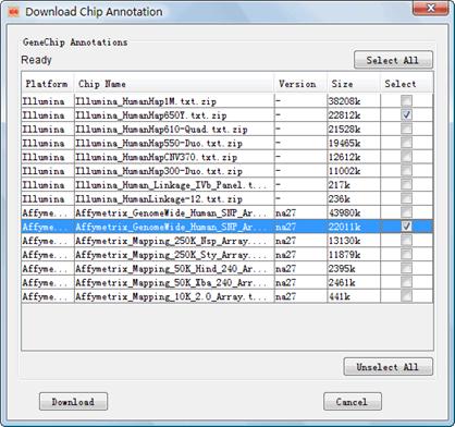
Figure 2: Dialog box of ��Download Chip Annotation��
Hint: You need not use third-party tools to download the HapMap and Genechip annotation data from the IGG website because IGG has employed multi-task and resuming-broken download technologies to speed up the download.
3.3 Annotation Files for HapMap and General Genotypes
Analogously, you have to download the annotation data from IGG��s website before integrating HapMap and general genotype datasets into your project. The downloading dialog can be opened by clicking the main menu Tools->Download Hapmap Annotation (Figure 3). The annotation files can be shared by the integration of HapMap and general genotypes datasets. These annotation data include the physical positions, flanking sequences, and strand information for all available SNPs in the NCBI��s dbSNP database, separated by chromosomes in different files. Downloaded annotation files can be viewed in the ��Available Resources�� Viewer of the main frame.
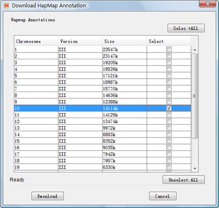
Figure 3: Dialog box of ��Download HapMap SNP Annotation��
4. Functions
IGG3 focuses on integrating huge among genotype data for meta-analysis and genotype imputation across genetic projects. The basic functions, including chip files integration, HapMap genotype integration, and exporting the integrated data for genetic analysis, are the same as previous versions. But by taking advantage of elegant computational technologies, it becomes feasible and very efficient to deal with tens of thousand of whole-genome samples on a popular desktop computer with memory less than 2 Gigabytes. These technologies are described in our new paper. Besides, IGG3 has introduced a Project-centered structure to clearly organize all involved data (Figure 4). Loaded pedigree file, chip types and genotype files are added into a project. Based on these loaded data, more than one ��Integration�� can be made and added into this project.

Figure 4: Project-centered data structure
4.1 Integrate Genotypes across various Chips
4.1.1 Create a Project
Compared with
previous versions, you need create a project before any integration on IGG3. A
click on the main menu File->Create Project or on the
accelerator![]() of the tool bar can open a dialog ��Create
an IGG Project�� (Figure 5). Explanations of settings on the dialog are list in
Table 1.
of the tool bar can open a dialog ��Create
an IGG Project�� (Figure 5). Explanations of settings on the dialog are list in
Table 1.

Figure 5: Dialog box of ��Create an IGG Project��
|
l Project Name: The name of the project l Project Path: Working path of this integration project. Integrated genotypes will be saved in this folder. l Specify phenotype names in pedigree files: Define one or more phenotypes in this project by clicking the + icon. Make sure the defined names are the same as those in your Chip Pedigree/subject File if you have. You will see the names when you export the genotypes for genetic analysis. |
Table 1: Explanations of settings on the dialog ��Create an IGG Project��
4.1.2 Load Genotype Datasets
4.1.2.1 Load Chip Genotype Files.
After creating the project, you can load the chip files into the project for
integration. The dialog, ��Load Chip Files�� (Figure 6) can be shown by clicking
either the
main menu File-> Load Chip Genotypes or the accelerator![]() on the tool
bar. Explanations
of settings on the dialog are list in Table 2.
on the tool
bar. Explanations
of settings on the dialog are list in Table 2.
Figure 6: The dialog of ��Load Chip Files��
|
l Platform: Choose a chip company name to show chip types. l Chip Type: Select a chip type to load chip genotype files l Load File: Load specific chip files of the selected chip types into the created project for integration. l Load Folder: Load all chip files of the selected chip types in a folder into the created project for integration. |
Table 2: Explanations of settings on the dialog ��Load Chip Files��
Hint: Ensure the loaded genotype files in the project have right chip types. A mismatch between the genotype files and chip types can result in loss of genotype data and even inconsistent genotypes in the integrated genotype sets.
4.1.2.2 Load Common Genotype Files.
Alternatively
you can load genotype datasets with a general format to integrate. The dialog, ��Load
Common Genetic Dataset�� (Figure 7) can be shown by clicking either the main menu File-> Load General Genotypes or the accelerator ![]() on the
tool bar. Explanations
of settings on the dialog are list in Table 3.
on the
tool bar. Explanations
of settings on the dialog are list in Table 3.
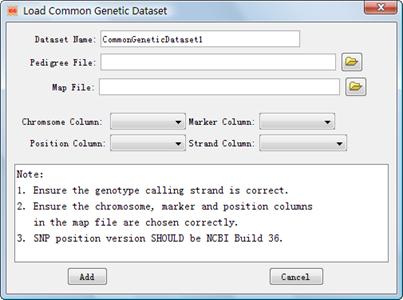
Figure 7: The dialog of ��Load Common Genetic Dataset��
|
l Dataset Name: Define a dataset name in the project. l Pedigree File: Choose pedigree file for the integration. See its format in 3.1.2.2. l Map File: Choose map file for the integration. See its format in 3.1.2.2. l Chromosome Column: A column in the map file to indicate the chromosome of a SNP. l Marker Column: A column in the map file to indicate the dbSNP RS-ID of a SNP. l Position Column: A column in the map file to indicate the physical postion of a SNP. l Strand Column: A column in the map file to indicate the strand of a SNP. Here you can also define that all genotypes in the pedigree file are called according to either the forward or the reverse strand. In this case the strand column in the map file can be omitted. |
Table 3: Explanations of settings on the dialog ��Load Common Genetic Dataset��
4.1.3 Integration Loaded Chip Genotype Files
After
loading the chip genotype files, you can start to integrate the genotypes. IGG3
provides two slightly different dialogs to launch two different integrations.
One dialog named ��Integrate Genotypes of Whole Genome�� (Figure 8) can be opened
by clicking the main menu Integrate->Whole Genome or the
accelerator![]() on the toolbar panel. This dialog is designed
to directly integrate available genotypes on the whole genome or chromosomes. Explanations
of settings on the dialog are list in Table 4.
on the toolbar panel. This dialog is designed
to directly integrate available genotypes on the whole genome or chromosomes. Explanations
of settings on the dialog are list in Table 4.
Figure 8: Dialog Box of ��Integrate Genotypes of Whole Genome��
|
l Name: Set a name to indentify the integration in a project. l Frequency Populations: Choose a reference population to output allelic frequencies in the final integration result. l Reserved Buffer Size: It is the maximal number of subjects processed by IGG at a time. The total times are equal to the smallest integer which is larger or equal to the quotient, total subjects number/buffer size. l Chromosomes: Specify chromosomes for the integration. The default setting is all chromosomes, i.e., the whole genome. |
Table 4: Explanations of settings on the dialog ��Integrate Genotypes of Whole Genome��
The other dialog was provided to integrate genotypes in certain regions rather than the whole genome (Figure 9). It can make a faster integration when you are only interested in genotypes within a specific and short region. This dialog can be shown by clicking the main menu Integrate ->Genome Region. Explanations of settings on the dialog are list in Table 4.
Figure 9: Dialog Box of ��Integrate Genotypes within Genomic Regions��
|
l Chromosomes of Genome: Choose chromosome(s) for the integration l Genetic Map Region: Set the region for the integration in terms of genetic map on selected chromosome(s). l Physical Region: You can set the region for the integration in terms of physical map (according to the reference genome) of selected chromosome(s). l Name: Set a name to indentify the integration. l Frequency Populations: Choose a reference population to output allelic frequencies in the final integration result. |
Table 5: Explanations of settings on the dialog ��Integrate Genotypes within Genomic Regions��
4.2 Integrate HapMap Unphased Genotypes into a Project
IGG3 can integrate both the
un-phased HapMap genotypes and the phased ones into local projects. Figure 10
shows the Dialog to integrate HapMap unphased genotype. This dialog can be
opened by clicking the main menu Integrate-> HapMap UnPhased Genotype
or accelerator![]() . Explanations of settings on the
dialog are list in Table 6.
. Explanations of settings on the
dialog are list in Table 6.
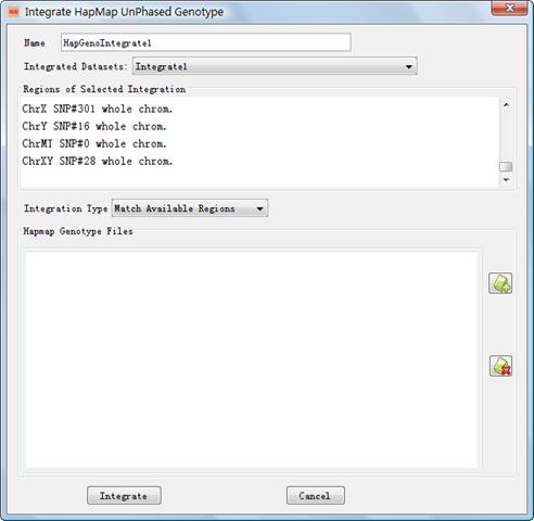
Figure 10: Dialog of ��Integrate HapMap Genotypes��
|
l Name: Name Set a name to indentify the integration l Integrated Dataset: Choose an available integration for the loaded chip files. The HapMap genotypes will be further merged with integrated genotypes in the selected integration. l Integration Type: Set an integration type, to match regions or only SNPs in the selected integration. ��Match Available Region�� selection means all HapMap genotypes in the region defined by a previous integration will be added; ��Match Available SNPs�� means IGG will only add HapMap genotypes of SNPs which exists in a previous integration. l HapMap Genotype Files: Click (figure+) to load HapMap genotype files for the integration. Conversely, click (figure-) to remove. The HapMap genotype files can be downloaded from http://ftp.hapmap.org/genotypes/?N=D. The downloaded files must be unzipped before loaded them into IGG. Please do not change the original filenames defined by HapMap. From these filenames IGG will automatically extract the chromosome, population, and strand information. Failure to get the information will result in a Java Exception to stop the integration. IGG assumes that all HapMap genotype files you loaded contain SNPs and genotypes on forward strand (according to the reference genome). The symbol ��fwd�� should appear in the filenames. Otherwise, the integrated genotypes may be not consistent between HapMap samples and the local project.
|
Table 6: Explanations of settings on the dialog ��Integrate HapMap Genotypes��
4.3 Integrate HapMap Phase Genotypes into a Project
Figure 11 shows the Dialog
to integrate HapMap phased genotypes into a project. This dialog can be opened
by clicking the main menu Integrate->HapMap Phased Genotype
or accelerator![]() . Explanations of settings on the
dialog are list in Table 7.
. Explanations of settings on the
dialog are list in Table 7.
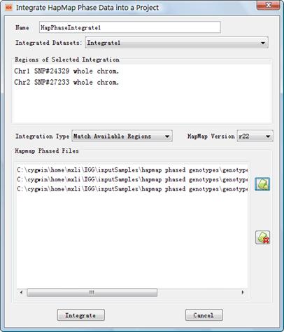
Figure 11: Dialog of ��Integrate HapMap Phased Genotypes��
|
l Name: The same as that in Table 6. l Integrated Dataset: The same as that in Table 6. l Integration Type: The same as that in Table 6. l HapMap Version: The same as that in Table 6. l HapMap Phased Files: Click (figure+) to add the HapMap phased files. Conversely, click (figure-) to remove. The HapMap phased genotype files can be downloaded from http://ftp.hapmap.org/phasing/?N=D. Again do not modify the filenames and ensure that genotypes loaded are on the forward strand (The symbol ��fwd�� should appear in the filenames). It should be noted that the phased HapMap genotypes released early have different format with the Phase 3. The early unphased HapMap genotype data are described by three complementary files, the phases, legend of phases and subject IDs corresponding to the phases. The names of these files end up with ��.phased��, ��_legend.txt��, and ��_sample.txt�� respectively for each population in each chromosome. IGG will check whether the sets of files are complete before integration. In contrast, the phased genotypes of Phase 3 only simply have one file for each population in each chromosome.
|
Table 7: Explanations of settings on the dialog ��Integrate HapMap Genotypes��
4.4 Export Integrated Datasets
4.4.1 Export Integrated Data for Routine Genetic Analysis
After
the integration, you can flexibly export the integrated dataset for a specific
statistical genetic analysis. A dialog ��Export Integrated Data for Genetic
Analysis�� (Figure 12) can be opened by a click on the menu Export ->Routine
Analysis or the accelerator![]() . Explanations of settings
on the dialog are list in Table 8.
. Explanations of settings
on the dialog are list in Table 8.

Figure 12: Dialog of ��Export Integrated Data for Routine Genetic Analysis��
|
l Integrated Datasets: Choose one dataset from available integrated datasets to export. l Phenotypes�� Ø Type: Choose the type of phenotypes in export output. There are three types of phenotypes, Quantitative Trait, Affection Status and Covariate. The three are usually differently treated by many tools. Ø Available: Phenotypes in the loaded pedigree file. Ø Selected: Phenotypes selected to export. l Filter: Ø Interval of Trimming: Set a length of intervals to trim the dataset. The default length is 0, indicating no trimming. The algorithm of trimming is very simple though very useful for genome-wide linkage scan. IGG first split the selected chromosomes or regions into even segments with the interval length customized. It then selects one SNP with the maximum heterozigosity on each segment for exporting (illustrated in Figure 13).
Figure 13: Algorithms to trim dataset Ø Remove Bad Mendel: IGG, once this setting is chosen, will automatically remove the genotype of a child if the Mendelian law is violated in a parents-child trio. Ø Remove All Missing SNPs: If the genotypes of an SNP are all missing, this SNP will be removed out of the exported dataset. Ø Correct Annotation Frequency (required for Linkage): Once selected, IGG will deal with the following situation. If a SNP has a zero allele frequency in the annotation file but has a non-zero one in the integrated datasets, IGG will replace the allele frequencies from the annotation file with the observed frequencies. This correction is necessary for many linkage tools. Otherwise, the linkage analysis may abort. l Files Ø Path: Set an output path for the exported files. Ø Prefix of FileName: Set the prefix names of exported files. l Format Ø Name of Tool: Popular tools for genetic analysis. Each tool has a special format. Once selected, IGG will generate a set of input files for the selected tool. Ø Missing Genotypes: A label denotes the missing genotypes in the output. It may vary from tools to tools although ��0�� is often used. Therefore, you��d better refer to document of the tools to set the missing genotype labels. Ø Strand: Control the genotype strand. This setting is effective only when the Numbered Allele checkbox is uncheckec. Ø Numbered Allele: Once this setting is checked, the format of output genotypes will be represented as numbers, 1 for allele A and 2 for allele B. l Specify Regions: It is an optional Setting. A click on this button will show a dialog to specify regions for exporting (Figure 14). The default setting will export all integrated genotypes. |
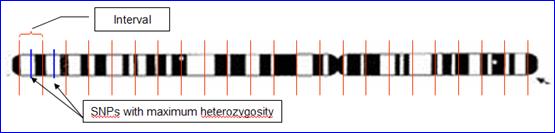
Table 8: Explanations of settings on the dialog ��Export Integrated Data for Routine Genetic Analysis��
Figure 14: Dialog of ��Specify Regions to Export Genotypes��
4.4.2 Export Integrated Data for Genotype Imputation
We separate genotype
imputation from routine genetic analysis by providing another dialog for
exporting. This dialog has fewer settings. Figure 15 shows the dialog which can
be launched through the man menu Export ->Genotype Imputation or
the accelerator![]() . Settings on this dialog have
the same meaning as the dialog on Figure 13. It is no need to explain them
again. IGG will run the following steps without asking you: remove the genotype
of a child once the Mendelian law is violated, delete SNPs whose genotypes are
all missing and not trim SNPs. Some imputation tools require phased data.
So you have to integrate HapMap phased genotypes if you want to export data for
these tools. Otherwise, you are not allowed to export integrated genotypes. At
the end of the integration, an example command will be suggested for you to run
the imputation tool being chosen with the input files generated by IGG. Here is
an example for IMPUTE (http://www.stats.ox.ac.uk/~marchini/software/gwas/impute.html):
. Settings on this dialog have
the same meaning as the dialog on Figure 13. It is no need to explain them
again. IGG will run the following steps without asking you: remove the genotype
of a child once the Mendelian law is violated, delete SNPs whose genotypes are
all missing and not trim SNPs. Some imputation tools require phased data.
So you have to integrate HapMap phased genotypes if you want to export data for
these tools. Otherwise, you are not allowed to export integrated genotypes. At
the end of the integration, an example command will be suggested for you to run
the imputation tool being chosen with the input files generated by IGG. Here is
an example for IMPUTE (http://www.stats.ox.ac.uk/~marchini/software/gwas/impute.html):
|
��An example command to run IMPUTE for genotype imputation on chromosome #: ./impute -h test.#.haplo -l test.#.legend -m genetic_map_chr#.txt -g test.#.geno -stest.#.strand -Ne 1100 -int postion1 postion2 -o test -i filename�� |
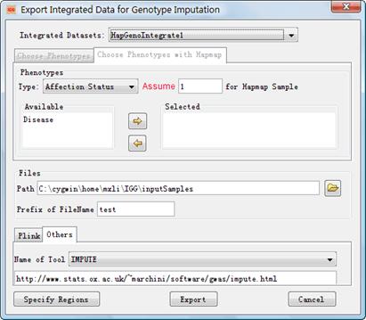
Figure 15: Dialog of ��Export Integrated Data for Genotype imputation��
5. Issues involving large datasets
As stated above, IGG of this version (3.0) is denoted to integrating whole genome genotypes across projects with large sample size and dense marker chips. Generally speaking, it requires less Random Access Memory (RAM) but runs much faster than previous versions IGG1 and IGG2 to deal with the same amount of genotypes. In addition, when the number of chip files is too large, IGG3 can automatically divide them into a number of groups and process the data group by group. When the sample is two large, say tens of thousands of arrays, you are suggested to set the maximum Java heap size (e.g. -Xmx1500m) as large as possible. The buffer size (Described in 4.1.3) will affect the speed of integration. The larger the buffer size, the faster the integration. But when the buffer size is too large, IGG will throw out an ��Out of Memory�� exception. The default buffer size is 2500, which is set for Affymetrix Genome-Wide Human SNP Array 6.0 and 1500MB Java heap size. You can set a larger number when chips to be integrated are smaller and/or your computer allows you set a larger Java heap size. Moreover, you can see a memory monitor in the graphic main frame to read the occupied memory during the process of integration. When there is still a lot of unused memory, the buffer size can be enlarged to deal with more chip files at a time. On the contrary, you need shrink the buffer size.
5.1 Testing Results as Reference
Several genotype datasets were generated to test the performance of IGG3. The datasets were made up of a number of virtual chip genotype files simulated for four large whole-genome chips: Affymetrix Genome-Wide Human SNP Array 6.0 and 5.0, Illumina Human1m-duo and Human650y-quad BeadChips. Under the continuous uniform distribution U(0,1), genotypes of SNPs were randomly assigned according to their available frequencies in the HapMap CHB+JPT population. Allele frequency 0.5 was set for SNPs without HapMap frequencies. The simulation function can also be launched by users on IGG3��s menu, Tools->Generate Sample. As a practical reference, the test was conducted on an ordinary desktop computer, Intel Core™ 2 Duo CPU 3.00GHz, RAM 2.00GB, and 32-bit Windows Vista™ Home Edition.
The running time and required RAM between IGG3 and IGG were compared to show how much improvement the new algorithm in IGG3 can achieve. IGG was originally designed for relatively modest chips like the Affymetrix Mapping 250K Nsp Array. It simply used characters to present genotypes and binary search method to locate a SNP in the annotation list, and had no adoption of the divide-and-conquer design. Table 9 shows the comparison results. IGG was found to work poorly in handling these large chips. Given the maximum RAM 1488 megabytes (MB), IGG could, at most, only integrate 120 subjects�� genotype chips (30 for each chip type) at a time. But IGG3 merely required 706 MB RAM to do this. More importantly, IGG3 ran over 10 times faster than IGG to integrate the whole genome genotypes. Furthermore, a huge dataset was used to test the performance of IGG3, 20,000 generated subjects�� genotype chips (5,000 for each chip type) and the HapMap (II+III) genotypes. The total size of the dataset was ~316.2 Gigabytes in the hard disk. This huge dataset could not be processed by IGG at all due to limited RAM on this ordinary computer. However, IGG3 still worked well in this situation (indicated by results in Table 9). We changed the buffer size from the default (2500) to 2000 as the larger number of SNP on Human1m-duo resulted in an ��Out of Memory�� exception.
|
|
120 Chips |
|
20000 Chips |
||||
|
|
R.RAM |
I.T. |
|
RAM |
I.T. |
H.U.T. |
H.P.T. |
|
IGG |
~1488MB |
~59.9min. |
|
Cannot be tested due to limited RAM |
|||
|
IGG3 |
~706 MB |
~5.4min. |
|
~1488MB |
~15.4hr. |
~16.4min. |
~12.9min. |
Table 9 Comparison of testing results between IGG and IGG3 for four popular large genotyping chips. Abbreviations: R.RAM: the required maximum RAM; min.: minutes; hr.: hours; I.T., H.U.T. and H.P.T.: the time to integrate all genotypes in the chips, the un-phased HapMap genotypes (CHB+JPT HapMap II+III) and the phased HapMap genotypes (CHB+JPT HapMap II) into chip genotypes respectively.
6. Problems and solutions
If you meet some problems when using IGG, please try following solutions before reporting errors to us.
1. Close and reopen IGG;
2. Reboot the computer. It will solve a lot of problems;
3. Make sure that a JRE is installed and running.
4. If you cannot see genotypes in the output of IGG, please check whether you have specified right Chip type of the genotype files.